Tutorial

This is a step-by-step tutorial for TARDIS analysis.

If you are new to TARDIS, we recommend you to follow this tutorial.*

Also, if you are new to spatial perturbation analysis, we recommend you to read the following paper:

Uncovering Spatially Resolved Functional Genomics with CRISPR Screen Sequencing.

Reference

SPAC-seq, the spatial transcriptomics based CRISPR screening technique, enables the direct linkage of genetic perturbation with spatially defined cellular microenvironments by integrating sgRNA reads with spatial transcriptomic profiles.

TARDIS represents the first dedicated software package designed specifically for spatial CRISPR screen analysis.

Preparations

Before everything, prepare your spatial CRISPR screen data.

Note

Although TARDIS is tested on multiple sequencing based spatial transcriptomics platforms, including BGI Stereo-seq, 10X Genomics Visium, and 10X Genomics Visium HD, and may not be limited to these platforms, it is still recommended to ensure that the data meets the following requirements:

• The data is spatially resolved. (e.g. Spatial barcodes are present)

• The data CAN BE from multiple tissues. (However, it is recommended to be preprocessed separately, and then combined into one AnnData object.)

• The data should contain guide annotation (e.g. Perturb-view) or guide UMI count matrix. (e.g. SPAC-seq)

TARDIS mainly integrates two forms of data to perform statistical analysis:

• Guide Mapping Data: Spatially resolved guide annotation or guide UMI count matrix.

• Spatial Transcriptomics Data: Spatial transcriptomics data.

In this tutorial, we will use the data from Uncovering Spatially Resolved Functional Genomics with CRISPR Screen Sequencing. The open-source data is available at Official SPAC-seq data repository.

In this set of data, we use two sets of data:

• BGI Stereo-seq data of a MC38 tumor, T cell infiltration perturbation library. (Library on SPAC-seq data repo: ‘Day7_rep1’)

  • Preprocessing and filtering

  • Bottom-up niche independent ranking of guides

• 10X Genomics Visium HD of subcutaneous mouse MC38 tumor, metastatic tumor cell perturbation library. (Library on SPAC-seq data repo: ‘Subq’)

  • Preprocessing and filtering

  • Clone calling for tumor models

  • Top-down niche dependent enrichment of guides

After downloading the data (or obtaining your own data), you can check on the data by loading the AnnData object.

Tip

Remember to move the data to the directory where you are running the code. Jupyter notebook is recommended for this tutorial.

import tardis_spac as td

Note

Import TARDIS using python, you can utilize scanpy, squidpy, numpy, matplotlib, seaborn, and pandas. scanpy and squidpy are required for spatial clustering analysis, numpy is required for numerical operations, matplotlib and seaborn are required for visualization, and pandas is required for data manipulation.

Infiltrated T cell library

In this section, we will perform TARDIS analysis on the infiltrated T cell library. This data is from BGI Stereo-seq platform.

Basic information of the data:

• The sample is sliced from a MC38 tumor, with perturbation of T cell injected, disected and sequenced on day 7 of tumor growth.

• The data contains 68 guides, with each perturbation of gene 2 different guide, 2 guides for non-targeting control.

TARDIS aims to pinpoint guides that have significant spatial difference of guide to non-targeting control guide, which reflects functional effect of the perturbed gene.

Loading and preprocessing

import tardis_spac as td
fdata = td.utils.load_data('Day7_rep1.guide.gem', bin_size=100)

AnnData object with n_obs × n_vars = 68003 × 68
obsm: 'spatial'

Note

The AnnData object contains the tissue Spatial Transcriptomics data and guide-targeting data. The obsm[‘spatial’] is the spatial coordinates of the data, which is used for spatial clustering analysis. The var_names is the variable names of the data, which is used for guide distribution analysis. The obs_names is the observation names of the data, which is used to contain the bin information

More information about the AnnData object can be found at [here](https://scanpy.readthedocs.io/en/stable/api/scanpy.AnnData.html).

In poly-A based SPAC-seq, guide count matrix is stored in ‘gem’ file. A gem file is a table file derived from the ‘gef’ file, which is the output of the BGI SAW software. (See here) A gem file is a tab-separated file with the following columns:

• index: the identical index of the guide detection

• guide: the guide name

• x: the x coordinate of the guide detection

• y: the y coordinate of the guide detection

• MIDCount: the guide count

• ExonCount: the detected exon count, usually same to MIDCount

We can read the gem file using pandas.

Note

gem file can be directly read by our module td.utils.load_bin() however, we will show you how to read the file using pandas for preprocessing.

Filtering and Quality Control

Spatial perturbation can be highly arbitrary if we cannot perform valid preprocessing and filtering of low quality guides and bins. Refer to Uncovering Spatially Resolved Functional Genomics with CRISPR Screen Sequencing for difference between filtered and unfiltered guide distribution.

TARDIS performs filtering with validation panels with the following methods.

# perform quality check from BGI stereo-seq GEM output
td.preprocess.filter_qc_bins('Day7_rep1.guide.gem')

The function processes a GEM file containing guide reads and performs filtering based on the specified parameters:

1. Reads the GEM file and optionally filters for guides with a specific prefix

2. Removes bins with guide counts below the threshold if specified

3. Handles bins with multiple guides according to the assign_pattern:

   • ‘max’: Keeps only the guide with highest count in each bin

   • ‘drop’: Removes all bins that have multiple guides

   • ‘all’: Keeps all guides in multi-guide bins

4. Optionally binarizes the counts (sets all to 1)

5. Returns filtered DataFrame or saves to file

import scanpy as sc
import anndata as ad
import pandas as pd
import matplotlib.pyplot as plt
import seaborn as sns

import numpy as np
from scipy import sparse

from tqdm import tqdm

Note

Above is a common practice to filter and QC the guide from GEM file. Here we read in the guide and RNA data from the h5ad file, which can be downloaded from the SPAC-seq data repository.

guide_adata = sc.read_h5ad('/home/wpy/stereoseq/tutorial/DATA/Day7_rep1.guide.h5')
rna_adata = sc.read_h5ad('/home/wpy/stereoseq/tutorial/DATA/Day7_rep1.h5')

rna_adata

AnnData object with n_obs × n_vars = 567178 × 13177
    obs: 'marker', 'n_genes'
    var: 'mt', 'mt-', 'gm', 'Rb', 'rik', 'n_cells'
    obsm: 'spatial'

guide_adata

AnnData object with n_obs × n_vars = 568003 × 34
    obs: 'marker'
    obsm: 'spatial'

guide_adata.obsm['spatial'] = np.concat([np.zeros((guide_adata.obsm['spatial'].shape[0], 1)), guide_adata.obsm['spatial'][:, 1].reshape(-1, 1), guide_adata.obsm['spatial'][:, 0].reshape(-1, 1)], axis=1)

filtered_guide_adata = filter_guide_reads_h5(
    guide_adata,
    guide_prefix='sg',
    binarilize=True,
    assign_pattern='max',
    filter_threshold=1,
)

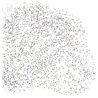
_, ax = plt.subplots(figsize=(5, 5))
td.utils.plot_spatial_guides(filtered_guide_adata, scale_factor=1, s=3, ax=ax)
ax.invert_yaxis()
plt.show()

filtered_guide_adata.var['n_total_counts'] = filtered_guide_adata.X.toarray().sum(axis=0)

sc.pl.highest_expr_genes(filtered_guide_adata, n_top=20, show=True)

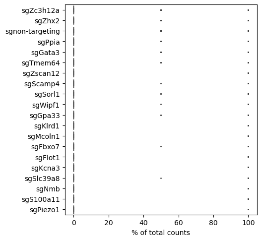
A robust CRISPR screening should have a good distribution of the guides with high expression.

Note

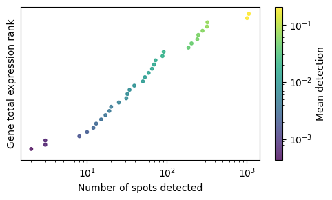
For robust ranking of spatially specific guides, an appropriate guide filter is essential. Based on data quality and cell type, we recommend a filter threshold of 200 for poly-A based SPAC-seq on T cells, as an example.

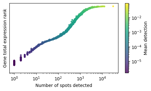
td.utils.plot_guide_gene_summary(filtered_guide_adata)

filtered_guide_adata = td.utils.combine_guide_replicates(filtered_guide_adata)

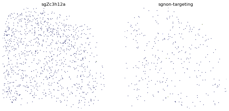
We can visualize the spatial distribution of the guides with high expression using td.utils.plot_spatial_guides().

Here we visualize the spatial distribution of the guides ‘sgZc3h12a’ and ‘sgnon-targeting’.

_, axs = plt.subplots(1, 2, figsize=(11, 5))
td.utils.plot_spatial_guides(filtered_guide_adata[filtered_guide_adata[:, 'sgZc3h12a'].X > 0], scale_factor=1, s=3, ax=axs[0])
axs[0].set_title('sgZc3h12a')
axs[0].invert_yaxis()
td.utils.plot_spatial_guides(filtered_guide_adata[filtered_guide_adata[:, 'sgnon-targeting'].X > 0], scale_factor=1, s=3, ax=axs[1])
axs[1].set_title('sgnon-targeting')
axs[1].invert_yaxis()
plt.show()

Kullback-Leibler divergence test

In cluster independent analysis, we perform KL divergence test to determine the guide specificity compared to non-targeting guide. Cluster independent means that we would like to know the guide specificity compared to wild type T cells.

Note

KL Distance Ranking is generally a method to model distribution of guides that have low spatial resolution or the spatial encoding is not the essential feature. As KL Distance Ranking dicards the spatial relationship between locations.

td.stats.kl_divergence(
    filtered_guide_adata,
    reference_guide='sgnon-targeting',
    result_field='kl_div',
    n_permutations=10000
)

/home/wpy/miniconda3/envs/tardis/lib/python3.14/site-packages/tqdm/auto.py:21: TqdmWarning: IProgress not found. Please update jupyter and ipywidgets. See https://ipywidgets.readthedocs.io/en/stable/user_install.html
  from .autonotebook import tqdm as notebook_tqdm
KL divergence permutations: 100%|██████████| 32/32 [01:00<00:00,  1.90s/it]

td.utils.plot_top_kde(
    filtered_guide_adata,
    result_field='kl_div',
    sgnt_label='sgnon-targeting',
    top_n=2,
)

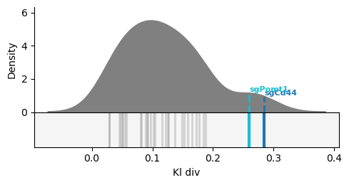
We can check the distribution of the guides with high KL distance. This function plot_ranking_scatter() is a simple function to plot the KL divergence test result using scatter plot to demonstrate the distribution of the guides with high KL distance.

td.utils.plot_ranking_scatter(filtered_guide_adata, 'sgnon-targeting', result_field='kl_div')

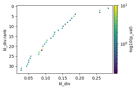
All KL distance results are stored in the adata.var attribute named ‘kl.div’ by default.

Warning

KL divergence test requires reference guide. Make sure to set the reference guide correctly using the reference_guide parameter. The reference guide can be set to ‘sum’ or ‘ntc’ (non-targeting control guide).

Perturbed subcutaneous tumor model

In this section, we will perform perturbed subcutaneous tumor model analysis.

We will use the perturbed subcutaneous tumor model data.

Note

In this part, we DID NOT perform Cellcharter analysis for spaitally awared clustering. Rather, we used graphclust clustering from Spaceranger output.

import tardis_spac as td

import scanpy as sc
import anndata as ad
import pandas as pd
import matplotlib.pyplot as plt
import seaborn as sns

import numpy as np
from scipy import sparse

from tqdm import tqdm

The following h5 files can be downloaded from above link.

guide_adata = sc.read_h5ad('filtered_guide_bc_matrix.h5')
rna_adata = sc.read_h5ad('filtered_gene_bc_matrix.h5')

/path/to/anndata/_core/anndata.py:1884: UserWarning: Variable names are not unique. To make them unique, call .var_names_make_unique.
  utils.warn_names_duplicates("var")

Make sure to make the variable names unique.

rna_adata.var_names_make_unique()

rna_adata

AnnData object with n_obs × n_vars = 632032 × 19059
    obs: 'in_tissue', 'array_row', 'array_col'
    var: 'gene_ids', 'feature_types', 'genome'
    obsm: 'spatial'

guide_adata

AnnData object with n_obs × n_vars = 632032 × 1520
    obs: 'in_tissue', 'array_row', 'array_col'
    var: 'gene_ids', 'feature_types', 'genome'
    obsm: 'spatial'

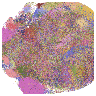
TARDIS provides a function td.utils.plot.plot_spatial_guides() to plot the spatial guides.

Note

Image can be provided together with scale_factor to plot the spatial guides on the HE for reference.

_, ax = plt.subplots(figsize=(5, 5))
td.utils.plot.plot_spatial_guides(guide_adata, scale_factor=scalefactors, s=1, ax=ax)
plt.show()

General quanlity control

guide_adata.var['n_total_counts'] = guide_adata.X.toarray().sum(axis=0)

sc.pl.highest_expr_genes(guide_adata, n_top=20, show=True)

/tmp/ipykernel_39694/2812346091.py:1: UserWarning: Some cells have zero counts
  sc.pl.highest_expr_genes(guide_adata, n_top=20, show=True)

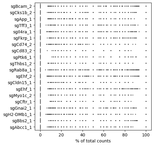
A robust CRISPR screening should have a good distribution of the guides with high expression.

td.utils.plot_guide_gene_summary(guide_adata)

Clone calling for tumor Models

In tumor models, we would like to call the clones from the spatial guides.

To identify clonal perturbations that locally expanded in the metastatic screen (defined as spatially proximal tumor bins with the same perturbation), ensity-based spatial clustering of applications with noise (DBSCAN) and kernel density estimation (KDE) were performed for each perturbation within each tissue section.

TARDIS provides a function td.utils.dbscan_density_region() to perform dbscan density region clustering.

Note

For recovery of larget clones, try raising the eps parameter. For recovery of small clones, try lowering the min_samples parameter.

Remember to tune eps according to the spatial resolution of the platform. For example, for 10x Visium data, eps should be set to 5-10. (~8 pixels per 2um bin)

perturb_data, perturb_points_df = td.utils.dbscan_density_region(
    guide_adata,
    "sgBcam_2",
    eps=20,
    min_samples=10,
    label="0",
    mode="most",
    density_level=7,
)

Number of Clusters (excluding noise): 25

We can visualize the clone calling result.

_, ax = plt.subplots(figsize=(5, 5))
sns.scatterplot(
    data=perturb_points_df,
    x="pxl_row_in_fullres",
    y="pxl_col_in_fullres",
    s=2,
    edgecolor="none",
    ax=ax,
)
plt.axis('off')
plt.show()

Here we call top 50 guides with high expression.

top_clones = guide_adata.var['n_total_counts'].nlargest(50).index.tolist()
perturb_points_merge_df = pd.DataFrame()
perturb_data_list = []
for clone in tqdm(top_clones):
    perturb_data, perturb_points_df = td.utils.dbscan_density_region(
        guide_adata,
        clone,
        eps=20,
        min_samples=10,
        label="0",
        mode="most",
        density_level=7,
    )
    perturb_data = perturb_data[perturb_data.obs['dbscan_cluster'] != '-1'].copy()
    perturb_data_list.append(perturb_data)
    perturb_points_df['clone'] = clone
    perturb_points_merge_df = pd.concat([perturb_points_merge_df, perturb_points_df])
perturb_points_merge_df.groupby('clone').size().sort_values(ascending=False)

100%|██████████| 50/50 [02:54<00:00,  3.49s/it]

clone
sgBcam_2        26779
sgApp_1         12063
sgCks1b_2       11448
sgTff3_1        10704
...
sgAnk_1          1284
dtype: int64

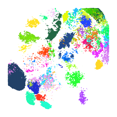
Visualize the clone calling result for top 50 guides with high expression.

_, ax = plt.subplots(figsize=(5, 5))
sns.scatterplot(
    data=perturb_points_merge_df,
    x="pxl_row_in_fullres",
    y="pxl_col_in_fullres",
    hue="clone",
    palette="gist_ncar",
    s=0.2,
    edgecolor="none",
    ax=ax,
    legend=False,
)
plt.axis('off')
plt.show()

Niche specific analysis

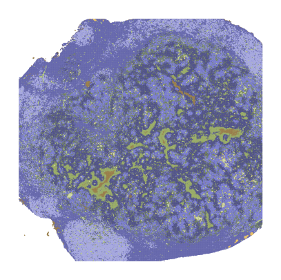
A tumor clone can be identified to be specificly distributed in a particular niche.

rna_adata.obs['graphclust'] = pd.read_csv('/path/to/spaceranger/output/outs/binned_outputs/square_008um/analysis/clustering/gene_expression_graphclust/clusters.csv', index_col=0)['Cluster'].astype(str)

_, ax = plt.subplots(figsize=(5, 5))
sns.scatterplot(
    data=rna_adata.obs,
    x='array_col',
    y='array_row',
    hue='graphclust',
    palette='tab20b',
    s=0.2,
    edgecolor="none",
    ax=ax,
    legend=False,
)
plt.axis('off')
plt.show()

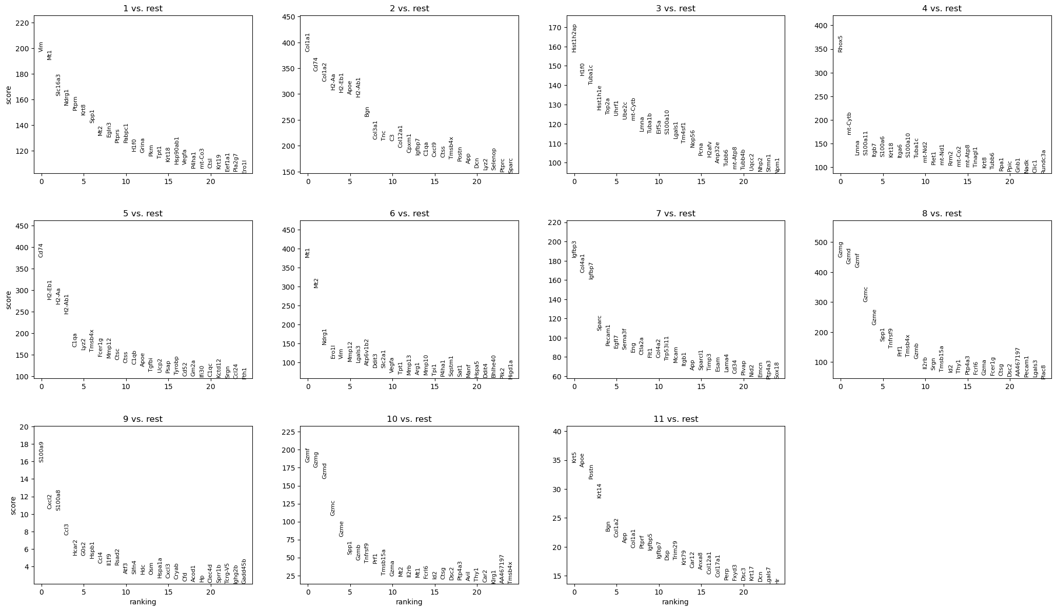
Define the niche by differential gene expression analysis.

sc.pp.normalize_total(rna_adata, inplace=True, target_sum=1e4)
sc.pp.log1p(rna_adata)
sc.tl.rank_genes_groups(rna_adata, 'graphclust', method='t-test')
sc.pl.rank_genes_groups(rna_adata, n_genes=25, sharey=False)

guide_adata.obs['graphclust'] = rna_adata.obs['graphclust']

perturb_data_merge = sc.concat(perturb_data_list)
perturb_data_merge = guide_adata[perturb_data_merge.obs_names.unique()].copy()

/path/to/anndata/_core/anndata.py:1882: UserWarning: Observation names are not unique. To make them unique, call .obs_names_make_unique.
  utils.warn_names_duplicates("obs")

Create a pseudo-guide, that is the sum of all the guides in the clone.

Warning

This is a very simple way to create a pseudo-guide, and may not be very accurate.

Due to limited detection of ‘sgNontargeting’ guide, we performed this simple method to create a pseudo-guide. It is recommended to use the ‘sgNontargeting’ guide for reference if detected.

if hasattr(perturb_data_merge.X, "toarray"):
    bin_sums = np.ravel(perturb_data_merge.X.sum(axis=1))
else:
    bin_sums = np.ravel(np.sum(perturb_data_merge.X, axis=1))

pseudo_adata = ad.AnnData(
    X=bin_sums.reshape(-1, 1),
    obs=perturb_data_merge.obs.copy(),
    var=pd.DataFrame(index=['sgPseudo'])
)

pseudo_adata = sc.concat([pseudo_adata, perturb_data_merge], axis=1)

pseudo_adata.obs['graphclust'] = rna_adata.obs['graphclust']

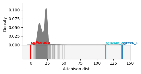
Calculate the Aitchison distance between the reference guide and the guides in the clone.

See td.stats.aitchison_distance() for more details.

td.stats.aitchison_distance(
    pseudo_adata,
    'graphclust',
    result_field='aitchison_dist',
    reference_guide='sgPseudo',
    n_permutations=None,
)

td.utils.plot.plot_top_kde(
    pseudo_adata,
    result_field='aitchison_dist',
    sgnt_label='sgPseudo',
    top_n=2,
)

TARDIS provides permutation test to calculate the p-value of the Aitchison distance.

Note

The p_swap parameter is the probability of swapping the guide labels. It is recommended to set to 0.5 for balanced data. For unbalanced data, it is recommended to set to 0.1-0.3.

filtered_guide_data = pseudo_adata[:, pseudo_adata.var_names.isin(top_clones + ['sgPseudo']).tolist()].copy()
filtered_guide_data.X = filtered_guide_data.X.astype(np.int64)

td.stats.aitchison_distance(
    filtered_guide_data,
    'graphclust',
    result_field='aitchison_dist',
    reference_guide='sgPseudo',
    p_swap=0.5,
    n_permutations=10000,
)

sgArf6_1: 100%|██████████| 10000/10000 [00:07<00:00, 1251.27it/s]
sgRab8a_1: 100%|██████████| 10000/10000 [00:08<00:00, 1247.24it/s]
sgCks1b_2: 100%|██████████| 10000/10000 [00:08<00:00, 1246.28it/s]
sgAgr3_2: 100%|██████████| 10000/10000 [00:08<00:00, 1246.10it/s]
...
sgTff3_1: 100%|██████████| 10000/10000 [00:08<00:00, 1247.87it/s]

Visualize the Aitchison distance scatter plot.

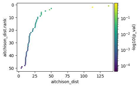
td.utils.plot_aitchison_dist_scatter(filtered_guide_data, 'sgPseudo')

[1]

He, P., Williams, B.A., Trout, D. et al. The changing mouse embryo transcriptome at whole tissue and single-cell resolution. Nature 583, 760–767 (2020).