Cellcharter

CellCharter-based Spatial Clustering

tardis_spac.external.cluster_cellcharter(adata, batch_key, n_clusters='auto', spatial_key='spatial', cluster_field='cluster', layer=None, random_seed=42, n_nodes_hidden_layers=32, dim_latent_layers=10, n_hidden_layers=5, gene_likelihood_model='poisson', latent_distribution='normal', save_model=None, use_model=None, inplace=True)

Perform joint spatial and expression-based clustering of spatial transcriptomics data using the CellCharter framework, integrated with scVI for representation learning and deep spatial feature aggregation.

Mathematical and Algorithmic Overview:

Latent Representation through scVI: - Gene expression profiles are integrated and batch-corrected using [scVI](https://docs.scvi-tools.org/), which employs a variational autoencoder (VAE). For observations (cells, beads, or bins) \(x_i\), scVI probabilistically encodes them as low-dimensional latent variables \(z_i\):

[
q(z|x) approx p(z|x)

] The objective is to maximize the variational lower bound of the marginal log-likelihood, providing a denoised, batch-effect-corrected latent space \(Z\).
Spatial Graph Construction: - Squidpy is used to build a spatial neighbor graph \(G = (V, E)\), typically using Delaunay triangulation based on the spatial_key coordinates. Each node represents a location/barcode; edges represent spatial adjacency.
Multi-Layer Neighborhood Aggregation (Feature Stacking): - CellCharter constructs higher-order neighborhoods by iterative aggregation over the spatial graph. For a given spot, the representation vector is iteratively augmented by summarizing (e.g., averaging) the features of its 1-hop, 2-hop, and up to n_layers spatial neighbors. This enables the integration of both intrinsic expression and local microenvironment context.
Clustering and Cluster Number Selection: - The aggregated feature matrix is clustered using methods such as k-means or Gaussian Mixture Models. If n_clusters is a range (tuple), CellCharter’s AutoK selects the optimal cluster number using criteria like BIC/AIC after running several seeds for stability. - The final cluster assignments are stored in adata.obs[cluster_field].

Biological Rationale and Application: - CellCharter enables the discovery of spatially and transcriptionally coherent “domains” or “microenvironments,” which may correspond to functional tissue niches, malignant subclones, immune cell pockets, or other spatial phenomena. - Its strength is the integration of both transcriptional state and spatial organization, providing robust clustering that can reveal structure invisible to expression-only approaches. - The approach is compatible with several spatial transcriptomics platforms, including Visium, Stereo-seq, Slide-seq, CosMx, etc. It is robust to batch effects and leverages both local and distant spatial context.

Parameters:

adata – AnnData object, containing both gene expression and spatial coordinates
batch_key – obs column specifying batch or sample identity for batch correction with scVI
n_clusters – Number of clusters (K); can be an int or a tuple (min, max) for automatic selection (‘auto’ = exhaustive selection in a user-range)
spatial_key – Key in adata.obsm that stores spatial coordinates (default “spatial”)
cluster_field – Name of the field in obs where cluster labels are saved (default “cluster”)
layer – AnnData layer to use as input (if None, use .X)
random_seed – Random seed for reproducibility (default 42)
n_nodes_hidden_layers – Number of nodes in scVI hidden layers (default 32)
dim_latent_layers – Number of latent dimensions for scVI (default 10)
n_hidden_layers – Number of hidden layers for scVI (default 5)
gene_likelihood_model – Gene likelihood function (default ‘poisson’)
latent_distribution – Latent distribution choice (default ‘normal’)
save_model – Whether or where to save the trained scVI model (bool or str path)
use_model – Use an existing saved scVI model (bool or str path)
inplace – If True, modifies adata in place; if False, returns a copy

Returns:

The processed AnnData object if inplace=False, otherwise None.

Example usage:

import tardis as td
# Perform CellCharter clustering, with automatic cluster number selection between 8 and 20
clustered_adata = td.external.cluster_cellcharter(
    adata,
    batch_key='batch',
    n_clusters=(8, 20),
    save_model='cellcharter_scvi_model.pkl'
)

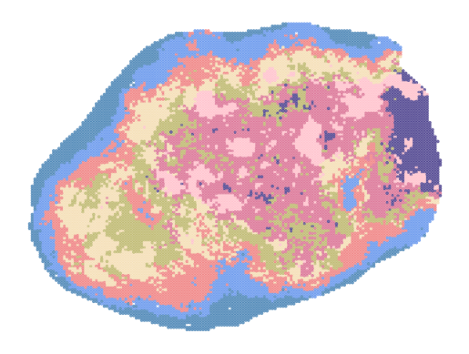
# Plot spatial clusters using seaborn
import seaborn as sns
n_clusters = clustered_adata.obs['cluster'].nunique()
palette = sns.color_palette('Set3', n_colors=n_clusters)
sns.scatterplot(
    x=clustered_adata.obsm['spatial'][:, 0],
    y=clustered_adata.obsm['spatial'][:, 1],
    s=8,
    hue=clustered_adata.obs['cluster'],
    palette=palette,
    alpha=0.4,
    legend=False,
    edgecolor='none'
)

References: - [CellCharter Documentation](https://cellcharter.readthedocs.io/en/latest/) - Vento-Tormo, et al. CellCharter: scalable and versatile clustering of spatial transcriptomics data. Nature Biotechnology, 2023.